
A step-by-step guide using PyTorch Geometric


Graph Neural Networks (GNNs) represent some of the fascinating and rapidly evolving architectures throughout the deep learning landscape. As deep learning models designed to process data structured as graphs, GNNs bring remarkable versatility and powerful learning capabilities.
Amongst the assorted sorts of GNNs, the Graph Convolutional Networks (GCNs) have emerged as probably the most prevalent and broadly applied model. GCNs are modern on account of their ability to leverage each the features of a node and its locality to make predictions, providing an efficient option to handle graph-structured data.
In this text, we’ll delve into the mechanics of the GCN layer and explain its inner workings. Moreover, we’ll explore its practical application for node classification tasks, using PyTorch Geometric as our tool of alternative.
PyTorch Geometric is a specialized extension of PyTorch that has been created specifically for the event and implementation of GNNs. It’s a sophisticated, yet user-friendly library that gives a comprehensive suite of tools to facilitate graph-based machine learning. To start our journey, the PyTorch Geometric installation will probably be required. When you are using Google Colab, PyTorch should already be in place, so all we’d like to do is execute a number of additional commands.
All of the code is accessible on Google Colab and GitHub.
!pip install torch_geometric
import torch
import numpy as np
import networkx as nx
import matplotlib.pyplot as plt
Now that PyTorch Geometric is installed, let’s explore the dataset we’ll use on this tutorial.
Graphs are a necessary structure for representing relationships between objects. You possibly can encounter graph data in a large number of real-world scenarios, similar to social and computer networks, chemical structures of molecules, natural language processing, and image recognition, to call a number of.
In this text, we’ll study the infamous and much-used Zachary’s karate club dataset.

The Zachary’s karate club dataset embodies the relationships formed inside a karate club as observed by Wayne W. Zachary through the Nineteen Seventies. It’s a sort of social network, where each node represents a club member, and edges between nodes represent interactions that occurred outside the club environment.
On this particular scenario, the members of the club are split into 4 distinct groups. Our task is to assign the proper group to every member (node classification), based on the pattern of their interactions.
Let’s import the dataset with PyG’s built-in function and check out to grasp the Datasets object it uses.
from torch_geometric.datasets import KarateClub
# Import dataset from PyTorch Geometric
dataset = KarateClub()# Print information
print(dataset)
print('------------')
print(f'Variety of graphs: {len(dataset)}')
print(f'Variety of features: {dataset.num_features}')
print(f'Variety of classes: {dataset.num_classes}')
KarateClub()
------------
Variety of graphs: 1
Variety of features: 34
Variety of classes: 4
This dataset only has 1 graph, where each node has a feature vector of 34 dimensions and is an element of 1 out of 4 classes (our 4 groups). Actually, the Datasets object could be seen as a set of Data (graph) objects.
We will further inspect our unique graph to know more about it.
# Print first element
print(f'Graph: {dataset[0]}')
Graph: Data(x=[34, 34], edge_index=[2, 156], y=[34], train_mask=[34])
The Data object is especially interesting. Printing it offers summary of the graph we’re studying:
x=[34, 34]is the node feature matrix with shape (variety of nodes, variety of features). In our case, it implies that we have now 34 nodes (our 34 members), each node being associated to a 34-dim feature vector.edge_index=[2, 156]represents the graph connectivity (how the nodes are connected) with shape (2, variety of directed edges).y=[34]is the node ground-truth labels. On this problem, every node is assigned to at least one class (group), so we have now one value for every node.train_mask=[34]is an optional attribute that tells which nodes must be used for training with an inventory ofTrueorFalsestatements.
Let’s print each of those tensors to grasp what they store. Let’s start with the node features.
data = dataset[0]
print(f'x = {data.x.shape}')
print(data.x)
x = torch.Size([34, 34])
tensor([[1., 0., 0.,  ..., 0., 0., 0.],
[0., 1., 0.,  ..., 0., 0., 0.],
[0., 0., 1.,  ..., 0., 0., 0.],
...,
[0., 0., 0.,  ..., 1., 0., 0.],
[0., 0., 0.,  ..., 0., 1., 0.],
[0., 0., 0.,  ..., 0., 0., 1.]])
Here, the node feature matrix x is an identity matrix: it doesn’t contain any relevant information concerning the nodes. It could contain information like age, skill level, etc. but this isn’t the case on this dataset. It means we’ll need to classify our nodes just by taking a look at their connections.
Now, let’s print the sting index.
print(f'edge_index = {data.edge_index.shape}')
print(data.edge_index)
edge_index = torch.Size([2, 156])
tensor([[ 0,  0,  0,  0,  0,  0,  0,  0,  0,  0,  0,  0,  0,  0,  0,  0,  1,  1,
1,  1,  1,  1,  1,  1,  1,  2,  2,  2,  2,  2,  2,  2,  2,  2,  2,  3,
3,  3,  3,  3,  3,  4,  4,  4,  5,  5,  5,  5,  6,  6,  6,  6,  7,  7,
7,  7,  8,  8,  8,  8,  8,  9,  9, 10, 10, 10, 11, 12, 12, 13, 13, 13,
13, 13, 14, 14, 15, 15, 16, 16, 17, 17, 18, 18, 19, 19, 19, 20, 20, 21,
21, 22, 22, 23, 23, 23, 23, 23, 24, 24, 24, 25, 25, 25, 26, 26, 27, 27,
27, 27, 28, 28, 28, 29, 29, 29, 29, 30, 30, 30, 30, 31, 31, 31, 31, 31,
31, 32, 32, 32, 32, 32, 32, 32, 32, 32, 32, 32, 32, 33, 33, 33, 33, 33,
33, 33, 33, 33, 33, 33, 33, 33, 33, 33, 33, 33],
[ 1,  2,  3,  4,  5,  6,  7,  8, 10, 11, 12, 13, 17, 19, 21, 31,  0,  2,
3,  7, 13, 17, 19, 21, 30,  0,  1,  3,  7,  8,  9, 13, 27, 28, 32,  0,
1,  2,  7, 12, 13,  0,  6, 10,  0,  6, 10, 16,  0,  4,  5, 16,  0,  1,
2,  3,  0,  2, 30, 32, 33,  2, 33,  0,  4,  5,  0,  0,  3,  0,  1,  2,
3, 33, 32, 33, 32, 33,  5,  6,  0,  1, 32, 33,  0,  1, 33, 32, 33,  0,
1, 32, 33, 25, 27, 29, 32, 33, 25, 27, 31, 23, 24, 31, 29, 33,  2, 23,
24, 33,  2, 31, 33, 23, 26, 32, 33,  1,  8, 32, 33,  0, 24, 25, 28, 32,
33,  2,  8, 14, 15, 18, 20, 22, 23, 29, 30, 31, 33,  8,  9, 13, 14, 15,
18, 19, 20, 22, 23, 26, 27, 28, 29, 30, 31, 32]])
In graph theory and network evaluation, connectivity between nodes is stored using quite a lot of data structures. The edge_index is one such data structure, where the graph’s connections are stored in two lists (156 directed edges, which equate to 78 bidirectional edges). The rationale for these two lists is that one list stores the source nodes, while the second identifies the destination nodes.
This method is often called a coordinate list (COO) format, which is actually a way to efficiently store a sparse matrix. Sparse matrices are data structures that efficiently store matrices with a majority of zero elements. Within the COO format, only non-zero elements are stored, saving memory and computational resources.
Contrarily, a more intuitive and easy option to represent graph connectivity is thru an adjacency matrix A. It is a square matrix where each element Aᵢⱼ specifies the presence or absence of an edge from node i to node j within the graph. In other words, a non-zero element Aᵢⱼ implies a connection from node i to node j, and a zero indicates no direct connection.

An adjacency matrix, nonetheless, isn’t as space-efficient because the COO format for sparse matrices or graphs with fewer edges. Nonetheless, for clarity and straightforward interpretation, the adjacency matrix stays a preferred alternative for representing graph connectivity.
The adjacency matrix could be inferred from the edge_index with a utility function to_dense_adj().
from torch_geometric.utils import to_dense_adj
A = to_dense_adj(data.edge_index)[0].numpy().astype(int)
print(f'A = {A.shape}')
print(A)
A = (34, 34)
[[0 1 1 ... 1 0 0]
[1 0 1 ... 0 0 0]
[1 1 0 ... 0 1 0]
...
[1 0 0 ... 0 1 1]
[0 0 1 ... 1 0 1]
[0 0 0 ... 1 1 0]]
With graph data, it is comparatively unusual for nodes to be densely interconnected. As you possibly can see, our adjacency matrix A is sparse (crammed with zeros).
In lots of real-world graphs, most nodes are connected to only a number of other nodes, leading to a lot of zeros within the adjacency matrix. Storing so many zeros isn’t efficient in any respect, which is why the COO format is adopted by PyG.
Quite the opposite, ground-truth labels are easy to grasp.
print(f'y = {data.y.shape}')
print(data.y)
y = torch.Size([34])
tensor([1, 1, 1, 1, 3, 3, 3, 1, 0, 1, 3, 1, 1, 1, 0, 0, 3, 1, 0, 1, 0, 1, 0, 0,
2, 2, 0, 0, 2, 0, 0, 2, 0, 0])
Our node ground-truth labels stored in y simply encode the group number (0, 1, 2, 3) for every node, which is why we have now 34 values.
Finally, let’s print the train mask.
print(f'train_mask = {data.train_mask.shape}')
print(data.train_mask)
train_mask = torch.Size([34])
tensor([ True, False, False, False,  True, False, False, False,  True, False,
False, False, False, False, False, False, False, False, False, False,
False, False, False, False,  True, False, False, False, False, False,
False, False, False, False])
The train mask shows which nodes are purported to be used for training with True statements. These nodes represent the training set, while the others could be regarded as the test set. This division helps in model evaluation by providing unseen data for testing.
But we’re not done yet! The Data object has rather a lot more to supply. It provides various utility functions that enable the investigation of several properties of the graph. As an illustration:
is_directed()tells you if the graph is directed. A directed graph signifies that the adjacency matrix isn’t symmetric, i.e., the direction of edges matters within the connections between nodes.isolated_nodes()checks if some nodes are not connected to the remaining of the graph. These nodes are prone to pose challenges in tasks like classification on account of their lack of connections.has_self_loops()indicates if at the least one node is connected to itself. That is distinct from the concept of loops: a loop implies a path that starts and ends at the identical node, traversing other nodes in between.
Within the context of the Zachary’s karate club dataset, all these properties return False. This means that the graph isn’t directed, doesn’t have any isolated nodes, and none of its nodes are connected to themselves.
print(f'Edges are directed: {data.is_directed()}')
print(f'Graph has isolated nodes: {data.has_isolated_nodes()}')
print(f'Graph has loops: {data.has_self_loops()}')
Edges are directed: False
Graph has isolated nodes: False
Graph has loops: False
Finally, we will convert a graph from PyTorch Geometric to the favored graph library NetworkX using to_networkx. This is especially useful to visualise a small graph with networkx and matplotlib.
Let’s plot our dataset with a special color for every group.
from torch_geometric.utils import to_networkx
G = to_networkx(data, to_undirected=True)
plt.figure(figsize=(12,12))
plt.axis('off')
nx.draw_networkx(G,
pos=nx.spring_layout(G, seed=0),
with_labels=True,
node_size=800,
node_color=data.y,
cmap="hsv",
vmin=-2,
vmax=3,
width=0.8,
edge_color="grey",
font_size=14
)
plt.show()

This plot of Zachary’s karate club displays our 34 nodes, 78 (bidirectional) edges, and 4 labels with 4 different colours. Now that we’ve seen the essentials of loading and handling a dataset with PyTorch Geometric, we will introduce the Graph Convolutional Network architecture.
This section goals to introduce and construct the graph convolutional layer from the bottom up.
In traditional neural networks, linear layers apply a linear transformation to the incoming data. This transformation converts input features x into hidden vectors h through using a weight matrix 𝐖. Ignoring biases in the meanwhile, this could be expressed as:

With graph data, a further layer of complexity is added through the connections between nodes. These connections matter because, typically, in networks, it’s assumed that similar nodes usually tend to be linked to every aside from dissimilar ones, a phenomenon often called network homophily.
We will enrich our node representation by merging its features with those of its neighbors. This operation known as convolution, or neighborhood aggregation. Let’s represent the neighborhood of node i including itself as Ñ.

Unlike filters in Convolutional Neural Networks (CNNs), our weight matrix 𝐖 is exclusive and shared amongst every node. But there’s one other issue: nodes do not need a fixed variety of neighbors like pixels do.
How will we address cases where one node has just one neighbor, and one other has 500? If we simply sum the feature vectors, the resulting embedding h could be much larger for the node with 500 neighbors. To make sure a similar range of values for all nodes and comparability between them, we will normalize the result based on the degree of nodes, where degree refers back to the variety of connections a node has.

We’re almost there! Introduced by Kipf et al. (2016), the graph convolutional layer has one final improvement.
The authors observed that features from nodes with quite a few neighbors propagate far more easily than those from more isolated nodes. To offset this effect, they suggested assigning greater weights to features from nodes with fewer neighbors, thus balancing the influence across all nodes. This operation is written as:

Note that when i and j have the identical variety of neighbors, it’s corresponding to our own layer. Now, let’s see implement it in Python with PyTorch Geometric.
PyTorch Geometric provides the GCNConv function, which directly implements the graph convolutional layer.
In this instance, we’ll create a basic Graph Convolutional Network with a single GCN layer, a ReLU activation function, and a linear output layer. This output layer will yield 4 values corresponding to our 4 categories, with the best value determining the category of every node.
In the next code block, we define the GCN layer with a three-dimensional hidden layer.
from torch.nn import Linear
from torch_geometric.nn import GCNConv
class GCN(torch.nn.Module):
def __init__(self):
super().__init__()
self.gcn = GCNConv(dataset.num_features, 3)
self.out = Linear(3, dataset.num_classes)    def forward(self, x, edge_index):
h = self.gcn(x, edge_index).relu()
z = self.out(h)
return h, zmodel = GCN()
print(model)
GCN(
(gcn): GCNConv(34, 3)
(out): Linear(in_features=3, out_features=4, bias=True)
)
If we added a second GCN layer, our model wouldn’t only aggregate feature vectors from the neighbors of every node, but additionally from the neighbors of those neighbors.
We will stack several graph layers to aggregate increasingly more distant values, but there’s a catch: if we add too many layers, the aggregation becomes so intense that each one the embeddings find yourself looking the identical. This phenomenon known as over-smoothing and generally is a real problem when you’ve too many layers.
Now that we’ve defined our GNN, let’s write an easy training loop with PyTorch. I selected a daily cross-entropy loss because it’s a multi-class classification task, with Adam as optimizer. In this text, we won’t implement a train/test split to maintain things easy and concentrate on how GNNs learn as an alternative.
The training loop is standard: we attempt to predict the proper labels, and we compare the GCN’s results to the values stored in data.y. The error is calculated by the cross-entropy loss and backpropagated with Adam to fine-tune our GNN’s weights and biases. Finally, we print metrics every 10 epochs.
criterion = torch.nn.CrossEntropyLoss()
optimizer = torch.optim.Adam(model.parameters(), lr=0.02)
# Calculate accuracy
def accuracy(pred_y, y):
return (pred_y == y).sum() / len(y)# Data for animations
embeddings = []
losses = []
accuracies = []
outputs = []# Training loop
for epoch in range(201):
# Clear gradients
optimizer.zero_grad()    # Forward pass
h, z = model(data.x, data.edge_index)    # Calculate loss function
loss = criterion(z, data.y)    # Calculate accuracy
acc = accuracy(z.argmax(dim=1), data.y)    # Compute gradients
loss.backward()    # Tune parameters
optimizer.step()    # Store data for animations
embeddings.append(h)
losses.append(loss)
accuracies.append(acc)
outputs.append(z.argmax(dim=1))    # Print metrics every 10 epochs
if epoch % 10 == 0:
print(f'Epoch {epoch:>3} | Loss: {loss:.2f} | Acc: {acc*100:.2f}%')
Epoch   0 | Loss: 1.40 | Acc: 41.18%
Epoch  10 | Loss: 1.21 | Acc: 47.06%
Epoch  20 | Loss: 1.02 | Acc: 67.65%
Epoch  30 | Loss: 0.80 | Acc: 73.53%
Epoch  40 | Loss: 0.59 | Acc: 73.53%
Epoch  50 | Loss: 0.39 | Acc: 94.12%
Epoch  60 | Loss: 0.23 | Acc: 97.06%
Epoch  70 | Loss: 0.13 | Acc: 100.00%
Epoch  80 | Loss: 0.07 | Acc: 100.00%
Epoch  90 | Loss: 0.05 | Acc: 100.00%
Epoch 100 | Loss: 0.03 | Acc: 100.00%
Epoch 110 | Loss: 0.02 | Acc: 100.00%
Epoch 120 | Loss: 0.02 | Acc: 100.00%
Epoch 130 | Loss: 0.02 | Acc: 100.00%
Epoch 140 | Loss: 0.01 | Acc: 100.00%
Epoch 150 | Loss: 0.01 | Acc: 100.00%
Epoch 160 | Loss: 0.01 | Acc: 100.00%
Epoch 170 | Loss: 0.01 | Acc: 100.00%
Epoch 180 | Loss: 0.01 | Acc: 100.00%
Epoch 190 | Loss: 0.01 | Acc: 100.00%
Epoch 200 | Loss: 0.01 | Acc: 100.00%
Great! Without much surprise, we reach 100% accuracy on the training set (full dataset). It implies that our model learned to appropriately assign every member of the karate club to its correct group.
We will produce a neat visualization by animating the graph and see the evolution of the GNN’s predictions through the training process.
%%capture
from IPython.display import HTML
from matplotlib import animation
plt.rcParams["animation.bitrate"] = 3000
def animate(i):
G = to_networkx(data, to_undirected=True)
nx.draw_networkx(G,
pos=nx.spring_layout(G, seed=0),
with_labels=True,
node_size=800,
node_color=outputs[i],
cmap="hsv",
vmin=-2,
vmax=3,
width=0.8,
edge_color="grey",
font_size=14
)
plt.title(f'Epoch {i} | Loss: {losses[i]:.2f} | Acc: {accuracies[i]*100:.2f}%',
fontsize=18, pad=20)fig = plt.figure(figsize=(12, 12))
plt.axis('off')anim = animation.FuncAnimation(fig, animate,
np.arange(0, 200, 10), interval=500, repeat=True)
html = HTML(anim.to_html5_video())
display(html)

The primary predictions are random, however the GCN perfectly labels every node after some time. Indeed, the ultimate graph is identical because the one we plotted at the tip of the primary section. But what does the GCN really learn?
By aggregating features from neighboring nodes, the GNN learns a vector representation (or embedding) of each node within the network. In our model, the ultimate layer just learns use these representations to supply the most effective classifications. Nonetheless, embeddings are the actual products of GNNs.
Let’s print the embeddings learned by our model.
# Print embeddings
print(f'Final embeddings = {h.shape}')
print(h)
Final embeddings = torch.Size([34, 3])
tensor([[1.9099e+00, 2.3584e+00, 7.4027e-01],
[2.6203e+00, 2.7997e+00, 0.0000e+00],
[2.2567e+00, 2.2962e+00, 6.4663e-01],
[2.0802e+00, 2.8785e+00, 0.0000e+00],
[0.0000e+00, 0.0000e+00, 2.9694e+00],
[0.0000e+00, 0.0000e+00, 3.3817e+00],
[0.0000e+00, 1.5008e-04, 3.4246e+00],
[1.7593e+00, 2.4292e+00, 2.4551e-01],
[1.9757e+00, 6.1032e-01, 1.8986e+00],
[1.7770e+00, 1.9950e+00, 6.7018e-01],
[0.0000e+00, 1.1683e-04, 2.9738e+00],
[1.8988e+00, 2.0512e+00, 2.6225e-01],
[1.7081e+00, 2.3618e+00, 1.9609e-01],
[1.8303e+00, 2.1591e+00, 3.5906e-01],
[2.0755e+00, 2.7468e-01, 1.9804e+00],
[1.9676e+00, 3.7185e-01, 2.0011e+00],
[0.0000e+00, 0.0000e+00, 3.4787e+00],
[1.6945e+00, 2.0350e+00, 1.9789e-01],
[1.9808e+00, 3.2633e-01, 2.1349e+00],
[1.7846e+00, 1.9585e+00, 4.8021e-01],
[2.0420e+00, 2.7512e-01, 1.9810e+00],
[1.7665e+00, 2.1357e+00, 4.0325e-01],
[1.9870e+00, 3.3886e-01, 2.0421e+00],
[2.0614e+00, 5.1042e-01, 2.4872e+00],
...
[2.1778e+00, 4.4730e-01, 2.0077e+00],
[3.8906e-02, 2.3443e+00, 1.9195e+00],
[3.0748e+00, 0.0000e+00, 3.0789e+00],
[3.4316e+00, 1.9716e-01, 2.5231e+00]], grad_fn=)
As you possibly can see, embeddings don’t must have the identical dimensions as feature vectors. Here, I selected to scale back the variety of dimensions from 34 (dataset.num_features) to 3 to get a pleasant visualization in 3D.
Let’s plot these embeddings before any training happens, at epoch 0.
# Get first embedding at epoch = 0
embed = h.detach().cpu().numpy()
fig = plt.figure(figsize=(12, 12))
ax = fig.add_subplot(projection='3d')
ax.patch.set_alpha(0)
plt.tick_params(left=False,
bottom=False,
labelleft=False,
labelbottom=False)
ax.scatter(embed[:, 0], embed[:, 1], embed[:, 2],
s=200, c=data.y, cmap="hsv", vmin=-2, vmax=3)plt.show()

We see every node from Zachary’s karate club with their true labels (and never the model’s predictions). For now, they’re all over because the GNN isn’t trained yet. But when we plot these embeddings at each step of the training loop, we’d have the ability to visualise what the GNN truly learns.
Let’s see how they evolve over time, because the GCN gets higher and higher at classifying nodes.
%%capture
def animate(i):
embed = embeddings[i].detach().cpu().numpy()
ax.clear()
ax.scatter(embed[:, 0], embed[:, 1], embed[:, 2],
s=200, c=data.y, cmap="hsv", vmin=-2, vmax=3)
plt.title(f'Epoch {i} | Loss: {losses[i]:.2f} | Acc: {accuracies[i]*100:.2f}%',
fontsize=18, pad=40)fig = plt.figure(figsize=(12, 12))
plt.axis('off')
ax = fig.add_subplot(projection='3d')
plt.tick_params(left=False,
bottom=False,
labelleft=False,
labelbottom=False)anim = animation.FuncAnimation(fig, animate,
np.arange(0, 200, 10), interval=800, repeat=True)
html = HTML(anim.to_html5_video())
display(html)
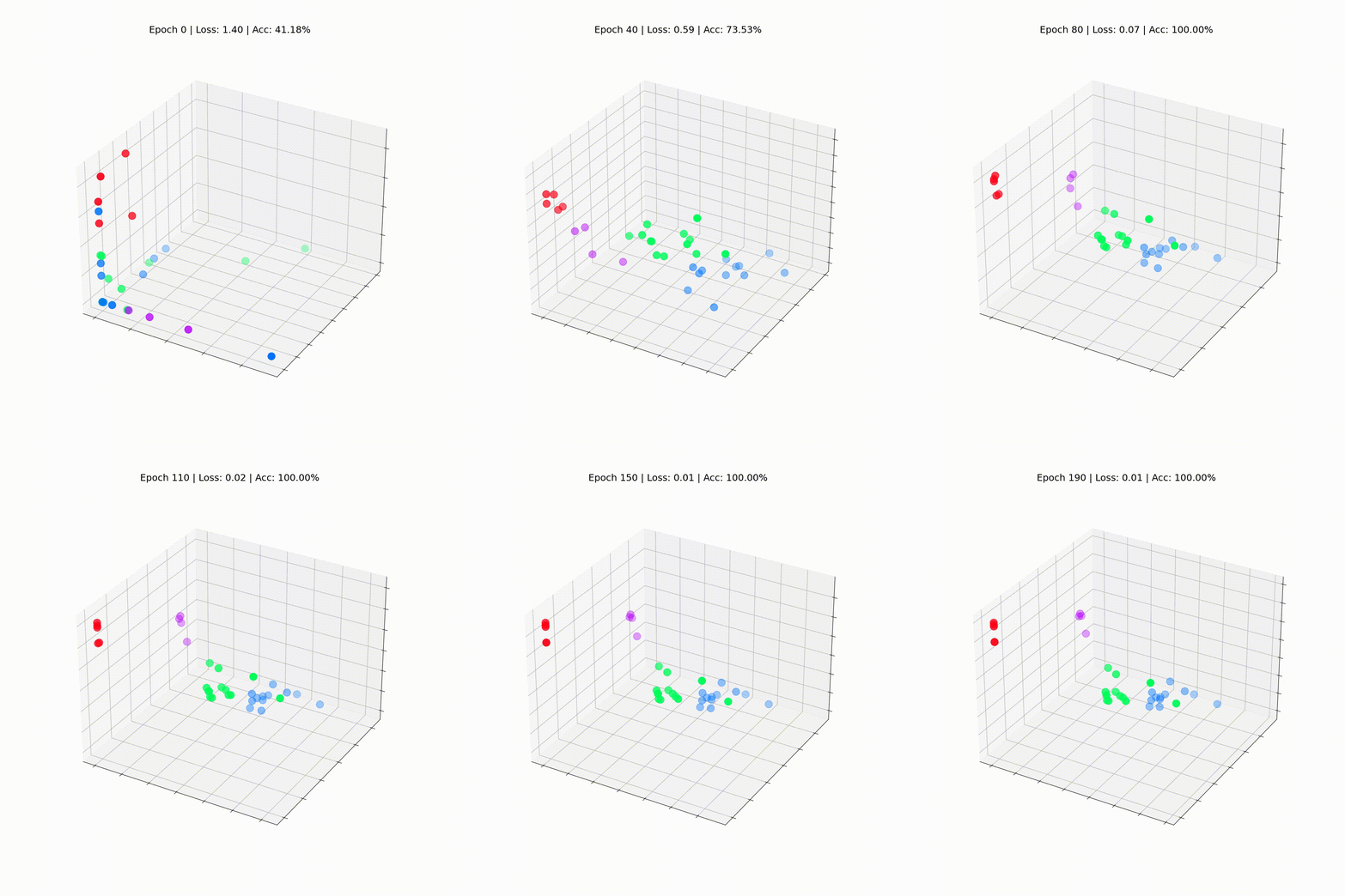
Our Graph Convolutional Network (GCN) has effectively learned embeddings that group similar nodes into distinct clusters. This permits the ultimate linear layer to differentiate them into separate classes with ease.
Embeddings are usually not unique to GNNs: they could be found all over the place in deep learning. They don’t need to be 3D either: actually, they rarely are. As an illustration, language models like BERT produce embeddings with 768 and even 1024 dimensions.
Additional dimensions store more details about nodes, text, images, etc. but in addition they create greater models which can be harder to coach. For this reason keeping low-dimensional embeddings so long as possible is advantageous.
Graph Convolutional Networks are an incredibly versatile architecture that could be applied in many contexts. In this text, we familiarized ourselves with the PyTorch Geometric library and objects like Datasets and Data. Then, we successfully reconstructed a graph convolutional layer from the bottom up. Next, we put theory into practice by implementing a GCN, which gave us an understanding of practical elements and the way individual components interact. Finally, we visualized the training process and obtained a transparent perspective of what it involves for such a network.
Zachary’s karate club is a simplistic dataset, but it surely is sweet enough to grasp an important concepts in graph data and GNNs. Although we only talked about node classification in this text, there are other tasks GNNs can accomplish: link prediction (e.g., to recommend a friend), graph classification (e.g., to label molecules), graph generation (e.g., to create recent molecules), and so forth.
Beyond GCN, quite a few GNN layers and architectures have been proposed by researchers. In the subsequent article, we’ll introduce the Graph Attention Network (GAT) architecture, which dynamically computes the GCN’s normalization factor and the importance of every reference to an attention mechanism.
If you would like to know more about graph neural networks, dive deeper into the world of GNNs with my book, Hands-On Graph Neural Networks.